Deep learning has shown huge advances in model architectures and techniques in the last couple of years, with transformers being in the center of attention when it comes to sequence to sequence tasks. Also, specific business cases demand more and more capabilities from such models, as people discover more ways to digest content.

Social media is the default option when it comes to ingesting news, especially in the form of videos. This type of media is present anywhere, from the standard YouTube to stories and tutorials, being easier to understand compared to written material. But since people have the urge to be more and more productive, they tend to prefer short video descriptions rather than consuming the whole input. Some of them might refer to this as the 80/20 principle, trying to get 80% of the video’s essence in a short paragraph, in just 20% of the time.

When trying to generate captions from videos, it seems that not only the visual information is important, but also the audio part. Similar to humans, the authors of the paper ‘A Better Use of Audio-Visual Cues’ exploit both modalities, generate some event proposals, and, with the filtered information they can generate captions. They use I3D and VGGish for the feature embedding, pass everything through normal self-attention layers and bi-modal attention and decode the results into words using GloVe. If you want to go directly to the fun part, scroll down for the Jupyter notebook that generates captions for YouTube videos.

For this to be possible, some nice deep learning methods have to be used. I’ll give a short sneak peek in this paragraph, then smoothly dive top-down in a comprehensive explanation. The goal is to take a video and generate a short, meaningful sequence and make it seem as if it was written by a human. In technical terms, that’s a sequence to sequence flow, since I take a time series, namely the video and transform it into a different type of sequential data, text.

This seems straightforward, but there are a few steps involved. To make this high-level flow easier to comprehend, let’s look at how humans do it. I look at a video, find the action-packed sections, and describe in natural language what happens there. Well, deep learning models must do the same thing. They take the video, find the action within, and then, for each of these sections, generate some representations. Consecutively, those are converted into actual words. What’s more, the method I’ll explain below focuses not limited to visual data but also uses the audio data from a video, so 2 modalities. It turns out that not only what I see has a meaning, but also what I hear, so deep learning models have to exploit this information as well, since, most of the time, a video has audio information as well.

In the following sections, I rely on the following paper: A Better Use of Audio-Visual Cues: Dense Video Captioning with Bi-modal Transformer. If the name does not make sense right now, that’s alright, I’ll split it into the following sections. Also, for simplicity, I’ll refer to this architecture/paper as BMT in the coming sections.

The part you’ve just read is the “Why” of the article, the reason for looking into such an approach for video-to-text translation. The following is structured as follows: In the “What” section I’ll dive deep into the paper and explain what they do. I’ll also draw parallels to existing methods for images and speech. Next, the “How” will cover specific implementation details and our work on top of this approach. Lastly, I’ll discuss the results and the importance of them and I’ll sum up all that’s been covered in the article.

BMT

As stated previously, the reference paper is BMT, or ‘A Better Use of Audio-Visual Cues: Dense Video Captioning with Bi-modal Transformer’. It was published quite recently, in May 2020 at the British Machine Vision Conference by 2 researchers at Tampere University in Finland. The title might seem confusing, so let’s break it down. The main contribution of the paper is that they do not only use visual cues, but also audio signals, hence the first part of the title. Afterward, they apply this for dense video captioning, with a transformer architecture that takes as input 2 modalities, you might guess, video and audio.

Main Idea

Their goal is 2 fold. First, they want to provide a transformer architecture that efficiently takes video and audio as input and provides accurate and meaningful embeddings. Then, using those generated vectors, they take their approach one step further and generate captions from untrimmed videos. Their ‘why’ is that generating meaningful descriptions from videos would be of high interest for many parties, such as recommendation systems, content retrieval engines, and, last but not least, direct consumers. They make a point specifically about visually impaired people. To make a short parallel, Facebook already does this with photos, generating some small captions to help in such cases, so making the step towards videos is the next natural move.

Their approach resembles the way humans think. They first locate the action in a video, then based on action-packed sequences generate embeddings and, ultimately, captions. The approach is straightforward because we’re so used to doing this in everyday life. On the technical side, though, things are a bit tangled since both audio and video signals have to work together towards creating qualitative results.

Related Work

Reading the paper, the main motivating factor for working on this problem is that previous work mostly focused on generating one caption for the whole video, which might not be the most insightful way of summarizing a, let’s say, 10-minute video. There might be multiple times where the action happens, so a more comprehensive description of the video might be worth the work. The word ‘dense’ in the title explains just this, compared to the ‘sparse’ approach previously taken.

There has been certainly tremendous work in this field before this paper, with the most noticeable areas being Transformers, Recurrent Neural Network architectures, and object detection using YOLO. I’ll further explain all these areas below so I provide a better understanding of how they relate to dense video captioning.

Video Captioning — overview

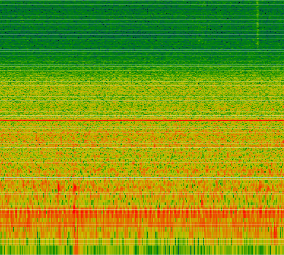
Before talking about generating text, let’s make sure I understand what a video is. In its most basic form, it’s a list of N images, most likely RGB, so 3 channels, C, with a set width W and height H. This yields a tensor of the shape of [N, C, W, H]. The audio sequences are represented as log mel-scaled spectrograms obtained via Short-time Fourier Transform. Although this might be a bit confusing, it’s out of the scope of this post to get into more details. What’s worth keeping in mind though is that those audio features are compressed into 128-dimensional features using VGGish.

On the video side, they use I3D, which stands for Inflated 3D Convolutional Nets (you can read more about this here), pretrained on the Kinetics dataset, which is a large scale dataset from DeepMind, with videos of the most common human to object and human to human interactions. This is of specific importance since it gives the captioning framework meaningful embeddings on what is happening in the video. Given the fact that I are interested in detecting the action in videos, I also need to know where the action happens, so I need some sort of flow detection in the video. For this, the authors use PWCNet (link) to extract the flow frames. On a high level, this network captures the action (or flow) in a sequence, exactly what I need for capturing the essence of a video.

Since I do a video to caption model, I also need a way to embed those output words. For this, the authors use GloVe embeddings, resulting in a feature vector of size 300 for each word in the output.

Comparison to simple video captioning

I think this comparison is valuable from 2 different points of view. First, as a direct consumer of such a video to caption model, I often look for information about multiple events of interest in the video and I would like, as much as possible, the caption to cover all of them. A model where just a shallow caption would be returned might not be enough for a good understanding of the video content, thus ‘simple video captioning’ might not be enough compared to ‘dense video captioning’.

On the technical side, simple video captioning would imply narrowing down the video to a few words sentence, without looking at the action-packed sequences, thus not extracting the full context. Instead, looking at the ‘information peaks’ might return more meaning in the generated captions.

YOLO — how it relates

I mentioned before that previous work is concerned with Yolo (You Only Look Once) for object detection. How does this relate to generating captions from videos? What Yolo does is generating a few proposals for objects within images. You might already see the common point. The paper I discuss does a similar thing, but instead of generating object proposals on each image, it generates action proposals for the whole video.

Event detection

Specifically, the method takes chunks of T frames and runs them through a simple multi-layer feed-forward network to generate the event proposals. Similar to how YOLO does it, they return the proposed regions together with a confidence score. Using this, they take the top 100 most confident predictions and cluster them using k-means. From this, they output the final event proposals to the next module, which is the decoder.

Caption generation per event

Here comes the more interesting part, the caption generation from video events. I have seen in previous work architectures that would take just video and, through a transformer, output a prediction. Here, their main differentiator is that they use both video and audio features, which have to be blended, as visible in this seemingly complicated architecture below. Let’s break it down.

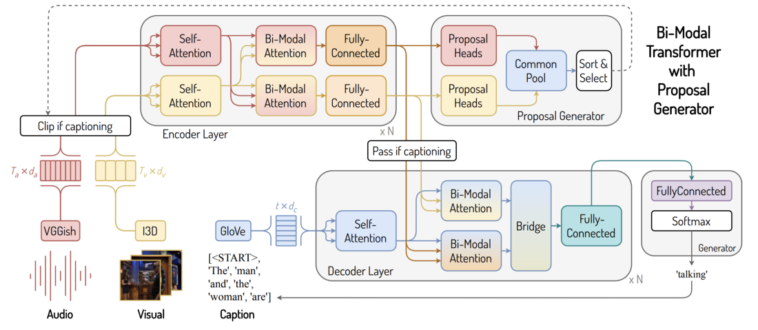
On the bottom left I have the input for the whole system, namely visual and audio features. Near them, I have the output, namely the captions. The fun part happens in between, where the bi-modal attention comes into play, among others.

First of all, starting with the raw features, I pass them through VGGish and I3D to get a lower-dimensional representation of the audio and video. Don’t worry, I dive a bit deeper into that in the next section. Then, I go through the Encoder layer, which squeezes as much information as possible from them, through regular self-attention (which acts only per modality) and with by-modal attention, which blends both modalities. In plain English, the video features borrow information from the audio, and the audio from the video features. After this knowledge transfer happened, everything is forwarded through some fully connected layers to get the features. Here the flow can take 2 ways. First, the system generates the regions of interest, what we’ve called before ‘event proposal’. With these, I can filter the stream of information and proceed to the captioning part. Here, I start decoding the information we’ve previously encoded, but now as word embeddings. Viewed from a high level, this is a translation task. I take videos and translate them to abstract space, from where I can decode them back to any format I want, in our case words. Having the generated captions I can easily convert them to words by using GloVe. That’s the architecture in a nutshell. Let’s dive even deeper into the technical details of this system.

Alright, let’s dive a bit deeper into this, and look a bit at the details of the techniques used in the BMT model.

This section is aimed to provide additional insight into the different concepts that are used in the paper. These will be the so-called feature embeddings and the transformer models.

Feature embeddings

As mentioned before, the BMT model relies on feature embeddings to function. From a high level, these embeddings can be thought of as a representation of the original data (or features). Often, these feature embeddings are used to encode high-dimensional data — such as audio and images — into a lower-dimensional space. The idea is then to have these lower-dimensional embeddings represent the important pieces of information of the original data. By doing so, the BMT model allows itself to get the original data encoded in a smaller number of parameters. For the BMT model three types of embeddings are used, the GloVe, VGGish, and I3D embeddings, for text, audio, and optical flow respectively. Let’s dive a little further into these embeddings.

GloVe

GloVe (short for Global Vectors) are representations for Words, from an unsupervised learning algorithm. In short, this unsupervised learning is performed by using global word-word co-occurrence statics (e.g. #co-occurences) to learn representations from a large text dataset — more generally known as a corpus (i.e. a body of words).

That’s a lot to take in one go, so let’s start with the most important part, word-word co-occurrence (statistics). I can think of this as a large matrix $W$with a row $i$ and a column $j$ for each word that occurs in a corpus. Then for every pair of words (wᵢ,wⱼ) in a word’s context, I increment the counters at the position Wᵢⱼ. The context is then defined as a window of n words around a word. For example with a window size of 6, the context for ‘defined’ would then be [context, is, then, as, a window]. From this matrix, an empirical estimate of a word j given i, i.e. Pᵢⱼ = P’ (j|i) = Wᵢⱼ / ∑ₖ Wᵢₖ — with a ’ to indicate that it is a measured statistic.

However, now I only have word statistics available. To convert these statistics to an actual embedding, the authors propose a series of numerical tricks to create an embedding that encapsulates the relation between words in a linear subspace. The details of this are out of scope for this post, but the original paper provides a nice explanation, and the Medium post by Jonathan Hui provides an excellent comparison of the different word embedding techniques. The important takeaway is that this embedding provides additional information about the context in which words are used, thereby providing additional information to the Decoder module.

In the BMT model, these embeddings are used in the Decoder layer, whhcih uses self attention on the GloVe embeddings generated by the Generator (note, not the Proposal Generator!). The decoder needs some initial ‘start’ data, in order to know that it start generate sentences, which is done by providing a (effectively gargabe) <START> token. They then iteratively predict a word to add to the description. This prediction is done by the Generator, which predicts with of the m words should be chosen. This m reflects the number of unique words in the training vocabulary, as such the model cannot predict words that did not occur in the training phase. Then the GloVe embedding of the predicted word is added to the input for the Decoder (plus a position encoding, because the self-attention is permutation invariant). However, how do I then decide when the caption is complete? For that I use a similar trick as for the <START> token, but I allow the Generator to predict <END_OF_SENTENCE>.

VGGish

VGGish was proposed by Hershey et al. (hershey2017cnn), which is VGG like CNN trained to classify audio. In addition, they apply some tricks to generate embeddings with this classifier. Let’s first consider how this VGG convolutional network is trained on audio data. To make the audio data compatible with a visual-oriented framework, so-called Logarithmic Mel spectrograms (Log-Mel) are generated from the audio data. This model was then pre-trained on the AudioSet, created by Google Research. Per its training regime, the network accepts data that corresponds to 0.96 seconds in a video (AudioSet consists of YouTube videos) and learns to predict the corresponding labels.

BMT, however, doesn’t need pre-classified audio, but representations, so how can I obtain those? The idea is relatively simple, I use the output of the second-to-last layer as a hidden (or deep) representation, i.e. embedding, of the input audio fragment.

Why would I do that? Let’s consider the architecture of the VGGish network, and specifically the last two layers. Both are fully connected layers, followed by a non-linearity, such as ReLU and the sigmoid. The ReLU, or Rectified Linear Unit, effectively ‘clamps’ the output of a layer at 0, effectively implementing the max operator for each output node. This non-linearity is used by all but the last layer of the VGGish network. During the training of this model, the last layer was followed by a Sigmoid σ(x) function, which turns the 3087 output features into logits (effectively turning the state of the output layer into probability scores).

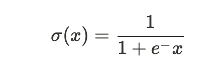
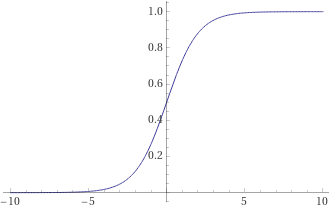
Sigmoid activation function, with curve on the right-hand side. Values of x close to zero are mapped close to 0.5, larger positive and negative values are mapped to 1 and 0 respectively.

To create actual embeddings, this last activation layer is dropped from the trained VGG model, and the output is multiplied with a matrix containing pre-computed principal components. Effectively this maps the hidden representation of the input onto the first 128 Principal Components of a large dataset, thereby reducing the output size from 3087 to 128. The model the authors of the BMT paper use was pre-trained by Google Research on the AudioSet. The PCA matrix is pre-generated by Google as well, which was achieved by performing PCA analysis on the hidden representations from a trained VGG model.

I3D

Inflated 3 Dimensional Convolutional neural networks can be seen as the way of allowing the capture of temporal events in a 2D CNN. Whereas a Recurrent Neural Network allows re-using its previous hidden state (see also the left architecture in the figure below), CNNs don’t have access to such previous information. However, by adding a dimension for time to our 2D convolution, I capable of ‘access’ information from previous frames. I must note that a 2D convolution also has a dimension for the number of channels of its input (e.g. RGB of an image), so effectively a 3D convolution spans 5 dimensions. From this, I can also see a clear disadvantage of the I3D architecture, it’s huge in terms of the number of parameters, and requires 8 GB of video memory to run inference on the GPU.

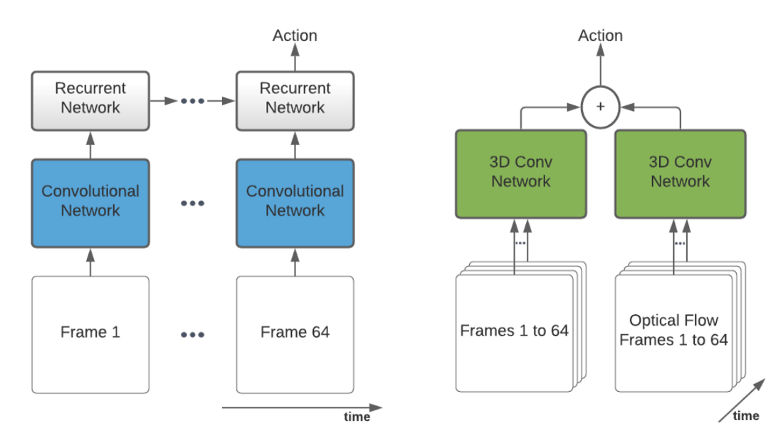
Similar to VGGish, I3D is trained to classify, however instead of classes of audio, classes of actions in videos. As such, the authors of BMT take the output of the ante-penultimate layer and use that as the embedding of a slice of a video. In BMT the authors by default sample the video at 25 fps, and their implementation of I3D expects 64 images (224x224 pixels), making that each embedding represents 64/24 ≈ 2.6 seconds of video.

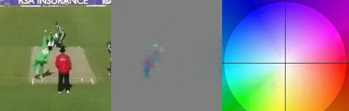
In the GIFs above I can see a small snippet of a cricket. Left I see the people playing, but on the right. The right represents the so-called optical flow, where for the sake of visualization colors are used to encode the x and y direction of individual pixels. If you look closely you can see that the colors of the pitcher’s arm at the start have the same color as the right-most player has after they start running.

The precise architecture of I3D and its training is outside of the scope of this blog post, but it is good to know where the optical flow images come from. In the original I3D paper, the authors use an implementation of the TV-L1 algorithm carreira2017quo (Total Variation decomposition with an L1 norm regularization). However, the author of this paper by default uses the PyTorch implementation of PWC nets by skiklaus. This is in favor of run-time and only needs to be done once for each inference (or training) sample.

Transformers

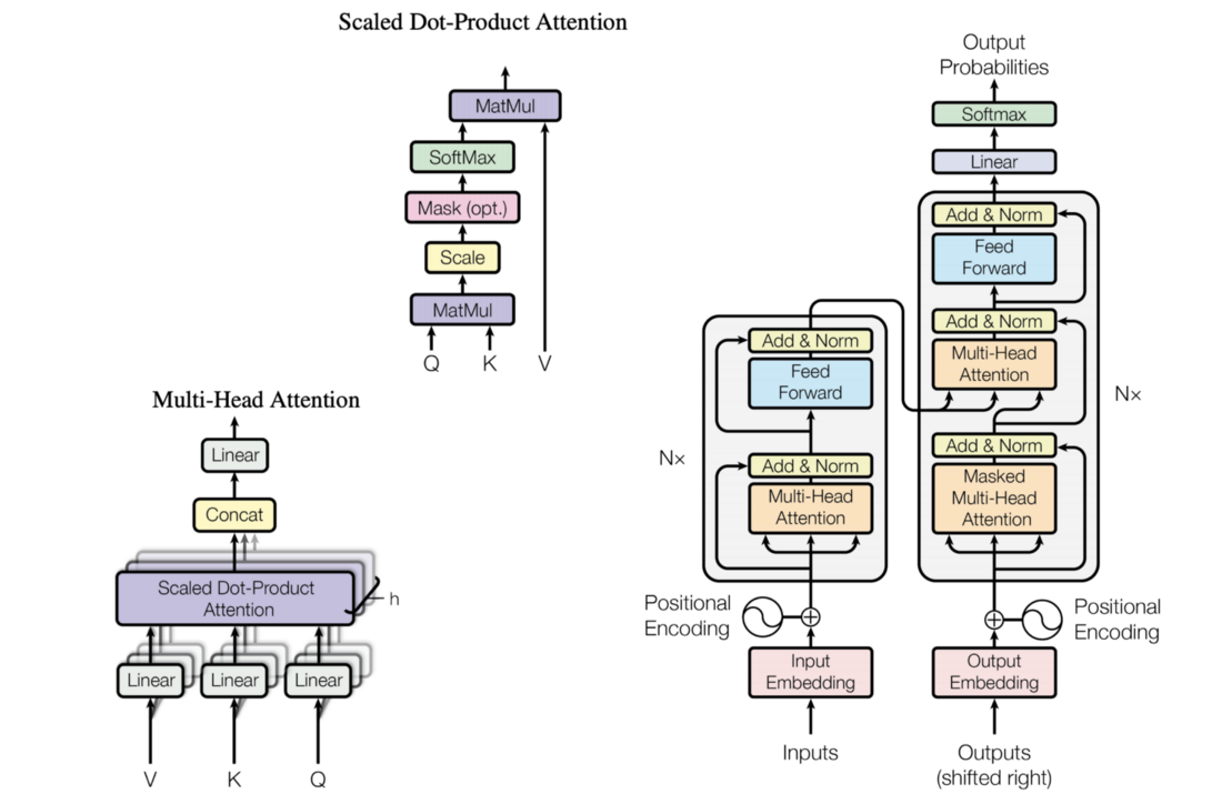
I think that for a better understanding of the paper I discuss, a detour to transformers and attention is needed. This architecture was introduced in 2017 by a paper called “Attention is all you need”. By introducing a new kind of sequence to sequence, named a transformer combined with a layer of attention, the authors of the paper, mostly from Google Research and Google Brain, were able to reduce the computational complexity and remove the convolutions and recurrences of the previous approaches. Through the attention mechanism, they have managed to link words together and transform standalone embeddings into embeddings that include context.

This does not take into account the temporal dimension, so they introduce some positional encodings to mitigate the issue. Otherwise, the same output could be reached by any random shuffle of the input sequence.

The architecture was initially designed for natural language translation, but it proved to be efficient in many other applications besides language to language translation.

Attention

This is where things get a bit fuzzy. Having a fixed-length sequence of embedded words, how do I re-weight them to get a sense of the context and find potential links they might form? This is what the attention mechanism does; at a very high level, it transforms each embedding into a more meaningful representation. This approach not only embeds the meaning of the word but also includes its context, which is a very important aspect when trying to figure out natural language or any other sequential data.

Going deeper into the technicalities of attention, I start with the embedding of each word. From this, I create 3 other learnable representations, the query, key, and value. The query of every word represents roughly how much it is interested in other words. The key, on the other side, is how much each word wants others to know about it. When I combine the query of the current word with the keys of every other word in the sequence I get a score. You can imagine this is a measure of the correlation between the words. Then, those scores are passed through a softmax layer so they roughly represent probability scores. Ultimately, the new representation of the current word becomes the linear combination between the scores and the value of each other word. The value is the most intuitive metric; it holds the gist, the signal of the word.

After doing all those computations, in parallel, I get the new embeddings for each word, but now context-aware. What we’ve just presented is called scaled dot-product attention, intuitively creating context on a single vertical. The paper uses multi-head attention, which is exactly the same thing, but with multiple attention heads, which might learn different perspectives of the context. One of such heads can thus dedicate itself to specific information in the input, independent of the other head. The exact number in the paper is 8 heads for their attention flow.

Transformer architecture

At the end of the day, the transformer has an encoder-decoder architecture, taking a sequence as input while predicting some probabilities on the other side. Because this complex architecture is created by stacking fully connected layers with attention layers, it provides maybe one of the main points of the paper, that of being able to train in parallel. This is a major string over Recurrent Networks, which depend on the output of a preceding prediction. (This can be alleviated somewhat with Teacher Forcing, but that is outside the scope of this blog).

Running it locally

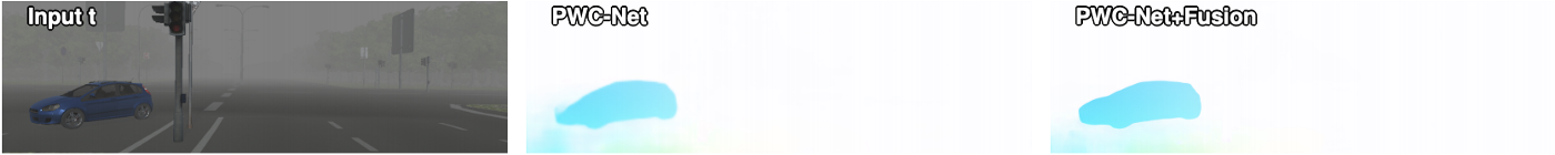
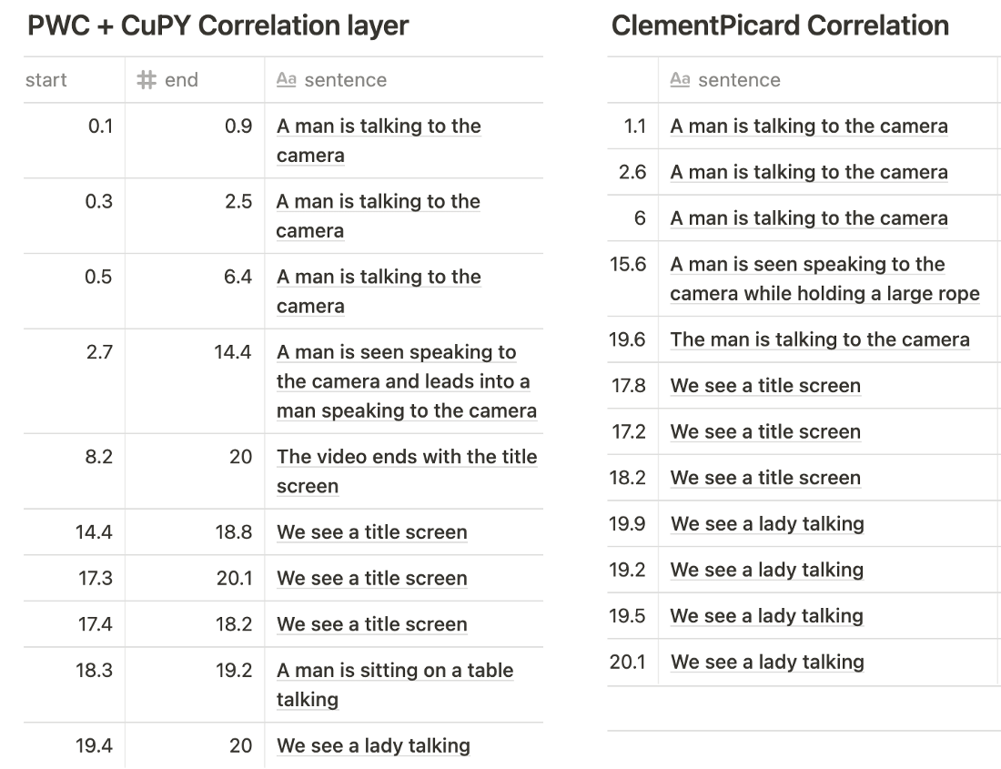
Our initial goal was to provide a local version of the captioning module, that would work with both CPUs and GPUs.Things went well when converting the captioning part since I only had to adapt the .cuda() calls, but on the feature generation side, I got stuck. This was because part of the used I3D feature extractor relied on code that was written in cupy, which involves low-level GPU code. Although possible, this proved to be not so straightforward to convert in plain PyTorch. Specifically, the PWC net's (to estimate the optical flow) Correlation function, not the sibling of the convolution operator. Other implementations that I found on GitHub made use of a library provided by Nvidia, which would not resolve the problem.

However, ClementPinard provided a custom PyTorch implementation of this correlation layer (see also this repo). I swapped the Correlation layer out with the implementation by ClementPinard in the PWC net that was used and compared the results with the original implementation. In the tables below I show the predictions generated by using the features extracted with I3D with the different PWC net implementations from the video below.

In addition, I ran a test on the CPU to see what speedup is gained by running the I3D feature generation on the GPU. Running the I3D extraction on CPU with an 18 seconds video took 167 seconds (4c/8t i7–7700 HQ). The GPU execution (Nvidia K80 on Google Collab) processes a 20-second video in about 16 seconds. That’s a speed-up of almost 12 times, however, this is not a fair comparison as the systems differ significantly (CPU system has an NVMe drive, whereas the Collab has an HDD), so this number should be taken with a grain of salt.

Updating dependencies

The BMT paper is mostly implemented in PyTorch. However, the VGGish network used was the original TensorFlow implementation. To circumvent this, the author proposes to use an adapter pattern, effectively wrapping the Tensorflow model inside a piece of code. However, this is written in the syntax of TensorFlow v1, which has received a major overhaul since the release of TensorFlow v2. As a result, when simply running pip install TensorFlow and trying to run the VGGish model, I were greeted by a serious list of exceptions. Although these were easily fixed by using the compat functionality of TensorFlow and adding a few additional dependencies. This, however, does not solve the problem, as the developers of TensorFlow may decide to drop the used functionality of compat, making the code not usable.

The second option would be to re-write the TensorFlow code in the newer syntax and re-generate the binary files that represent the learned parameters. I decided to go with the third option, re-creating the framework in PyTorch (check the repo). After figuring out the similarities between TensorFlow and Pytorch (spoiler: it’s in the ordering of dimensions), a conversion script was created that can convert a VGGish TensorFlow model into a BMT compatible VGGish PyTorch implementation. I also provide a download link for the converted models, but I also provided documentation for you to work with to convert your own VGGish TensorFlow model to PyTorch.

The implementation of the PyTorch was done to make the comparison with the original model more straightforward. To that end, the different layers follow the naming convention of the original model. The PostProcesssing module (the projection onto the 128 PCA vectors) is implemented as a Linear module (a classical Fully Connected Layer), which effectively implements the operation as a Matrix-Matrix product. However, this requires some care taken to make sure that I correctly subtract the mean from the features. By projecting the mean values onto the PCA dimensions, and flipping the sign (e.g. -1 → +1), the bias component of the Linear module can be used. By linearity, this provides the same result, in a neat one-liner (after conversion). As a result, the inference is faster as data does not need to be copied from a PyTorch Tensor to a NumPy Array, which saves a significant amount of time when data needs to be copied from GPU to CPU.

Similarly to when I changed the Correlation layer, I tested (again empirically) the difference in the generated captions. I found, however, that the generated captions were equivalent for the considered videos. In addition, I wrote a small smoke test that compares the outputs of the TensorFlow model.

From YouTube videos to captioning and visualization

Our end product, if you can call it so, is an end-to-end pipeline for generating captions. I use YouTube videos by default, but it can be extended to any type of video content or source. While reading this, I recommend opening this link and start running the cells. It takes quite some time for the first run, but hang tight. You’ll find instructions on how to run it in the notebook.

The flow is simple. I download the pre-trained models and the code, then download a video. (make sure you test on your content or videos that you have permission to download). The first step is to generate the video and audio features, as mentioned before in the article. Having those, I then do the inference and save the captions. With this, I can proceed and visualize some frames taken at equal intervals from each captions’ time window. This is more or less a metric for assessing the performance of the captioning system.

I think that the approach presented is especially useful for visually impaired people, but also for generic consumers that just need a video summary instead of spending the whole duration watching the movie.

Building an end-to-end pipeline for converting videos to captions is also useful, maybe not as a finished product, but as a proof of concept for sure. I also think that exploiting both modalities (video and audio) is very useful since it mimics how people do the same task. Also, looking into the action sections from a video provides a more accurate captioning mechanism, avoiding the redundant parts of a video.

I also worked with another dense caption model (DenseCap), which relies on the Caffe deep learning framework for generating features (Action recognition and optical flow). I dropped this idea in favor of BMT, as Caffe required a series of small changes to get started. As an alternative, a completely containerized environment could be created, but that would be more difficult to use for novice users that want to play with the code. In addition, I ran into a series of dependency issues, and deprecated functionalities. Again, containerization can alleviate this, but, unfortunately, work becomes harder to use due to frameworks or functions getting deprecated.

Lastly, I found that it was non-trivial to convert models that rely on GPU functionality to deploy locally, especially when only limited video memory is available. It is obvious that when research resources are available (e.g. high-end GPUs with copious amounts of video memory), that an (often much slower) CPU compatible variant is a low priority. However, this makes that research and state-of-the-art become less accessible to people with less powerful hardware.

To sum up, I provided a top-down approach in such an architecture, following a why-what-how structure, going from a bird’s eye view to the more fine-grained details. Make sure you check the repo(s) and also give the papers a read for more in-depth explanations of the topics. I know that there are a lot of third-party dependencies in this project, as a form of pre-trained models or techniques borrowed from other domains and I encourage you to explore them more by reading the papers or other blog posts.