Computer vision has been a hot topic for a long time, from cat and dog prediction to autonomous vehicles. There is a bit of AI in every product, materialized by deep learning models. Those are becoming better and better at their job, but since the data quantity evolves at a very fast pace, the training time and resources to make them work grow substantially.

The title might be a bit confusing; we will break it down later in the article. The mainline is: how can we semantically segment images and learn to do so without much input from humans?

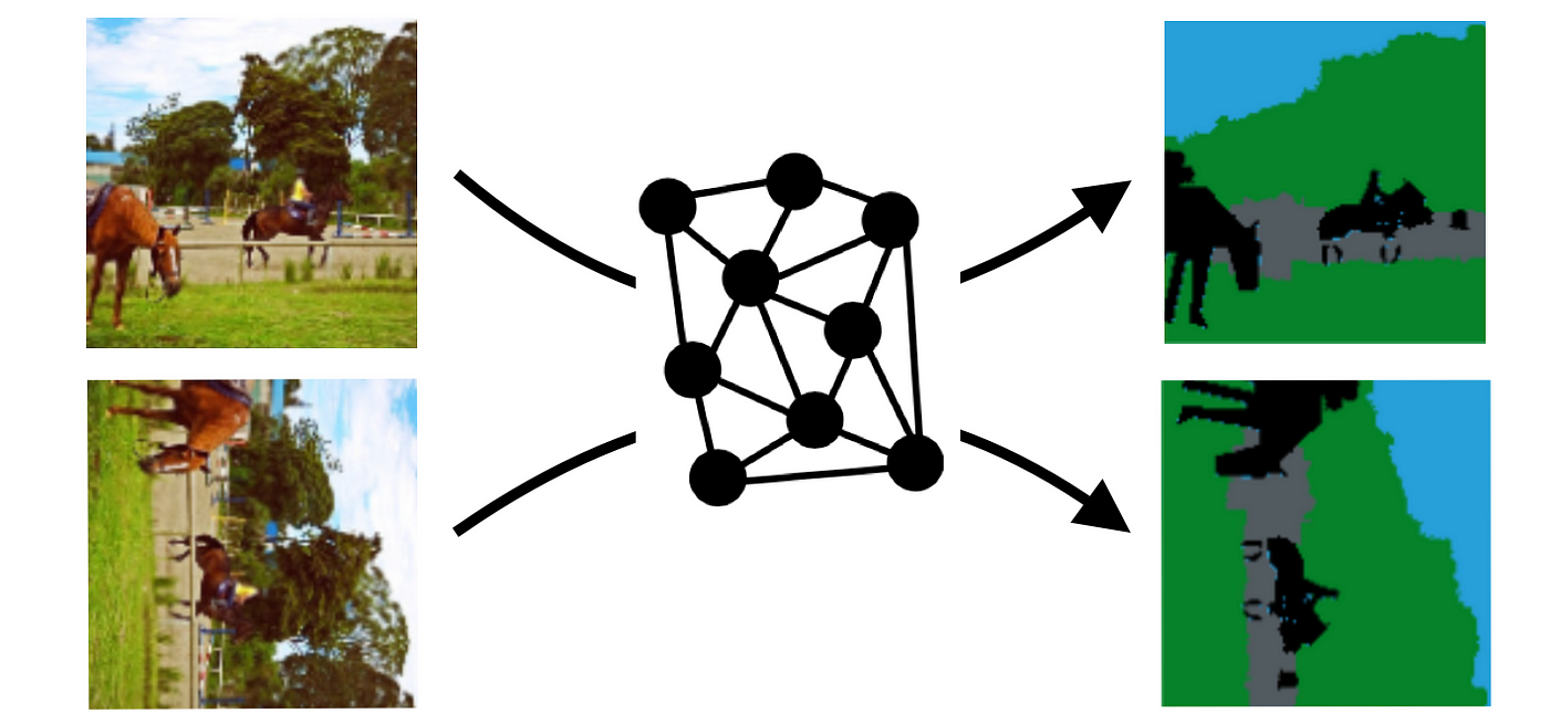
Image segmentation does not have to be expensive from a data annotation perspective. You can always generate controlled datasets by taking a list of images and define a set of revertible transformations. Ultimately, the goal of the paper is to remove the hassle of having to manually segment images for training. Instead, they use a simple network architecture together with the following hypothesis: having an image and a simple transformation, let’s say a 90° rotation, the output of the network should be the same, after reverting the rotation. The example below makes this a bit more clear.

This article was created by Anuj and me, Data Science Master’s students at TU Delft, aiming to introduce Invariant Information Clustering for Unsupervised Image Classification and Segmentation in a more casual style, diving deeper and deeper into the math and methodologies behind. We then also present our work and reproduced results.

Invariant Information Clustering for Unsupervised Image Classification and Segmentation, quite a long name, so we’ll refer to it as IIC from now on. IIC was published at International Conference on Computer Vision 2019 by 3 researchers from Oxford and provides novel image clustering and segmentation methods, aiming to reduce the labor of annotating each image, which is quite time consuming. This is called mutual information maximization and it learns what is that objects have in common, regardless of their position, orientation, or color scheme.

Let’s state some obvious facts to familiarise a bit with the domain of the problem. After building some domain knowledge, we’ll dive deeper into the Why, What and How of the paper, explaining the results in the end.

Image segmentation

An image is a collection of multiple pixels, each containing a numerical value ranging between 0–255 indicating how bright it needs to be and/or what color it needs to be, depending on the choice of representation space of the image (gray-scale gb gba). Segmentation deals with the task of partitioning complete images into separate clusters or segments based on what these segments represent.

While Classification deals with labelling images to separate datasets into categories and Object Detection deals with image localization by identifying the location of objects by creating bounding boxes around them, Segmentation goes a step further by increasing the granularity of what it achieves. Segmentation models provide the exact outline of the objects within an image by labelling each pixel with a probability value to belong to each category.

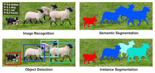
This blog post only talks about Semantic Segmentation, where all the pixels belonging to a particular class are represented by the same color, even if they represent different objects but belong to the same class.

Segmentation methods

Existing methods of Image Segmentation can be broadly divided into two branches: Image Processing based methods and Computer Vision based methods. Image Processing based methods deal with primitive processes where a fixed approach is used for all kinds of images for example Region-based and Edge-based segmentation methods. In Region-based segmentation, the pixel values are separated into categories using threshold values following the intuition that pixel values would vary drastically for objects belonging to different semantic classes. Edge-based segmentation methods use kernels that detect vertical and horizontal edges within images since different objects have an edge separating them. While these methods build on suitable reasoning and assumptions about images, these fail to perform well and generalize over a diverse set of complex and convoluted images where there is no significant gray-scale difference or an overlap of the gray-scale pixel values, or where there are several edges in an image.

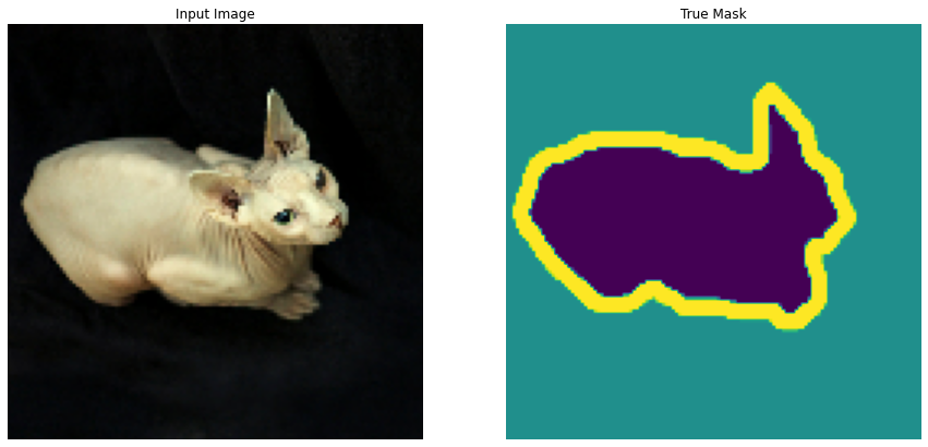
Computer vision based methods are fairly sophisticated in their approach and generalize well over large datasets too. These include supervised and unsupervised learning tasks to assign probability values to each pixel which indicate the class they belong to. Certain supervised image segmentation algorithms include Mask R-CNN and Auto Encoder based U-Net models. These take in the image as input and are trained against the true target classes of each pixel represented as masks. The trained models can then predict the masks for an image based on the total number of classes.

Real use-cases

Since segmentation achieves the exact outline of each object in an image, this high granularity in understanding object boundaries plays an extremely important part in tasks where detecting the shapes and details of objects is necessary.

A few real world use-cases of Image Segmentation are as follows — Traffic Control Systems in Self-Driving cars, Detecting Land bodies from Satellite Imagery, and Detection of Cancerous Cells where the shape plays a vital role in determining the malignity of the cells.

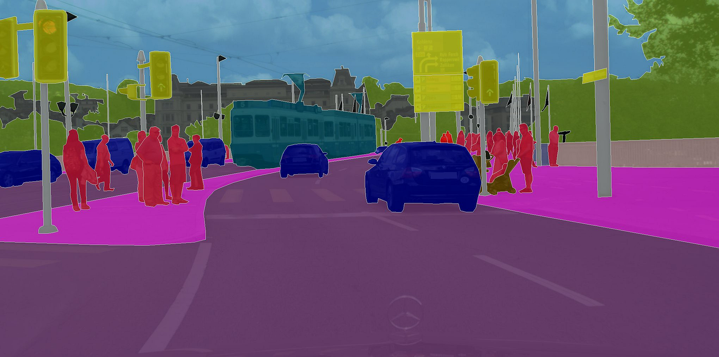
Object Localization and Segmentation to help self-driving cars make decisions by understanding the environment around them

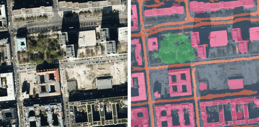
Semantic Segmentation of roads and residential areas using Satellite Imagery

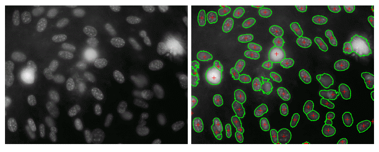
Cell Segmentation for cancer detection

Why unsupervised segmentation?

A common question that comes to mind when thinking about the need for this unsupervised approach is that — why even bother about trying to segment images in an unsupervised manner? Isn’t it an unnecessary complication to optimize for an information theoretical concept of mutual information just to solve a simple task of segmentation?

There are indeed a dozen extremely capable supervised algorithms that just need the image and its target masked output to train themselves to do this task over new images, but it is important to note that this class of algorithms requires the target annotation for each image. Supervised learning algorithms function on the concept of supervision, where the model must be provided with instances of the desired output to accurately learn a function that can replicate this behavior in the future, without supervision.

Unfortunately in our case of image segmentation, the costs of obtaining annotations in the form of masks for each image are exorbitant. Supervised learning algorithms require large labeled datasets to learn generalizable functions for optimal test performance, and the expensiveness of manually labeling images for segments largely limits their applicability in many scenarios.

This makes the need for the development of unsupervised methods that work just as well without target labels imperative.

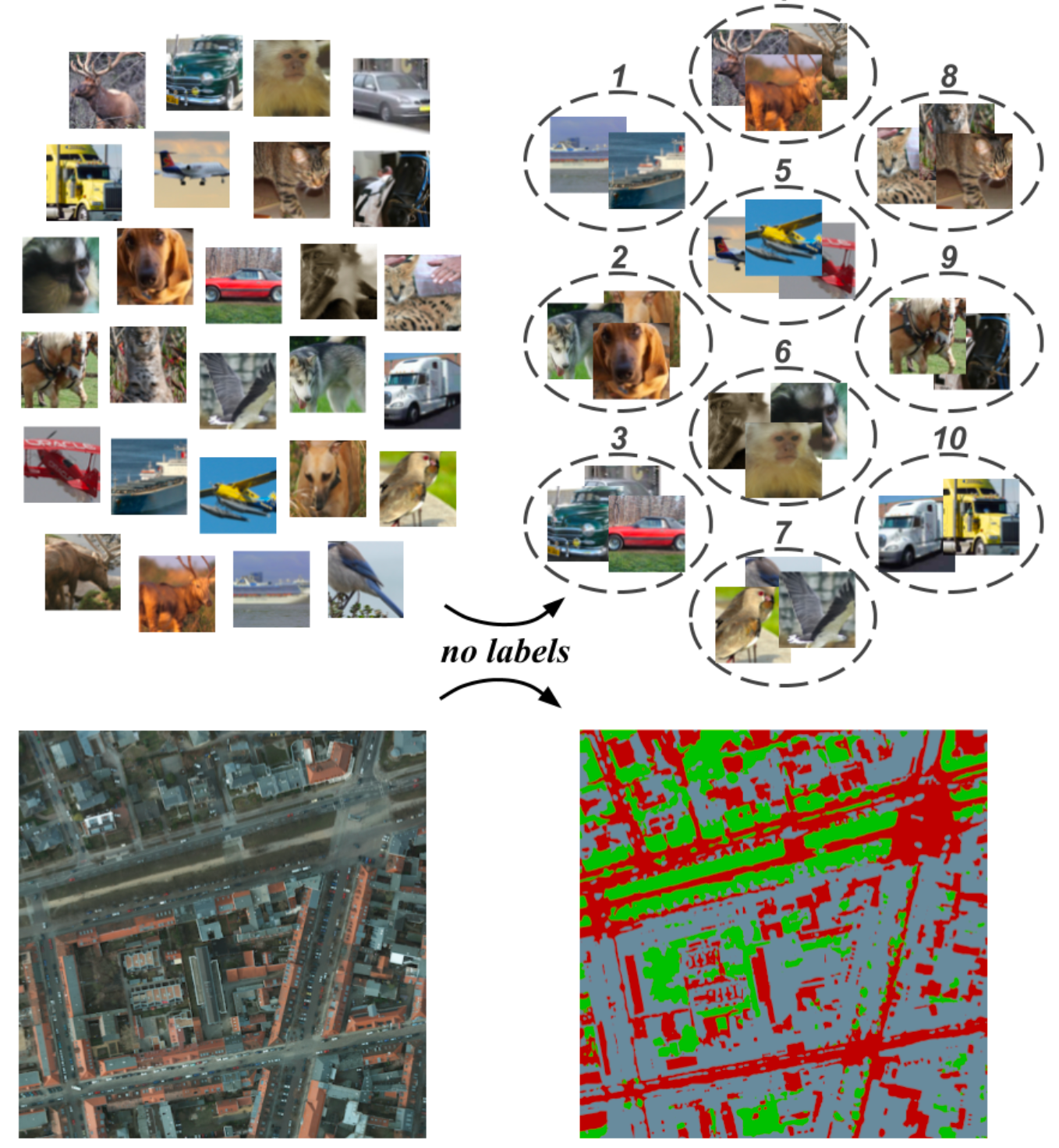
Imagine been given a task of clustering images together based on what their contents represent. Keep in mind that we have not been given any labels associated with these images that depict their content. A natural and valid approach to carry out this task with a human’s intuition would be to first identify the contents of each image and understand what they mean (which our brain does instantaneously), and then segregate them based on this contextual understanding.

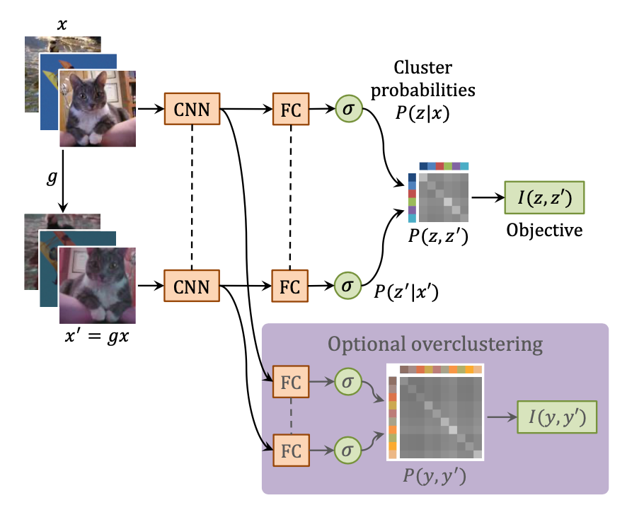
The authors translate this task into a machine understandable mathematical computation problem using the concept of Mutual Information. Mutual Information is a measure of the degree of mutual dependence between two random variables. It quantifies the amount of information obtained about one random variable by observing the other random variable. On an intuitive level, mutual information between two images indicates the amount of shared information between these 2 images. But to get an algorithm to pick out, then learn things and abstractions about similar images that maximize their mutual information measure, a Convolutional Neural Net is trained. The CNN is trained against a loss of function of maximizing mutual information between 2 similar images. The information that is fed to the mutual information function is the 2 vectors of probability values for each image, output by the CNN. The probability values are the probabilities of the images belonging to each class of the predefined clusters. It is important to note here that the CNNs used for computing the prob. vectors for image pairs share their weights.

As the saying goes, there’s no free lunch. Here the difficulty shifts from acquiring labels of images to acquiring other images similar to each image. But as some lunches are cheaper than others, it is easier to obtain images that are very similar to each other by the means of data augmentation techniques than obtain ground truth labels for each image. Image pairs are created by randomly perturbing the original images using any such perturbation that leaves the content of the image intact. To extend the application of this approach, it can be implemented on the scale of pixels inside images. The mutual information can be maximized between neighboring pixels after applying several convolution operations on them. The weights of these convolutional blocks would be adjusted by back-propagating the loss gradients over the entire function, to better represent each image pixel in the form of a probability valued vector over multiple classes.

To extend the application of this approach, it can be implemented on the scale of pixels inside images. The mutual information can be maximized between neighboring pixels after applying several convolution operations on them. The weights of these convolutional blocks would be adjusted by back-propagating the loss gradients over the entire function, to better represent each image pixel in the form of a probability valued vector over multiple classes.

Once the model learns over multiple data samples and several epochs of training, it assigns probability values to each pixel based on the similarity of content between patches, using the concept of maximizing mutual information between images.

The authors introduce a novel objective/loss function to be optimized, to learn a neural network classifier from scratch in an unsupervised manner.

The Invariant Information Clustering (IIC) algorithm aims to learn a parameterized representation of the image that preserves common information between the image pairs and discards irrelevant instance-specific information.

Clustering and Segmenting Images using unsupervised learning by maximizing invariant mutual information.

Thus the idea is to maximize the mutual information shared between the original and a randomly perturbed version of the image: max I(Φ(x), Φ(x’)), where Φ : x → y.

The parameterized representation of the image Φ is simply a convolutional neural network that converts the image into a vector of probability values using a softmax function in the output layer. Each element of the vector represents the probability of belonging to a target class.

x’ is the randomly perturbed version of the image where the perturbation x’ = g(x) is geometrically and photometrically invariant, for eg: scaling, skewing, rotation, flipping, contrast/saturation change, etc.

In simple English, this means that the perturbation must only change the geometric or photometric properties of the image without disturbing what the content of the image depicts.

IIC is then forced to recover the information which is invariant to the pair of images input to the neural network. The neural network acts as a bottleneck for the flow of information to the objective function and thus by training the model to maximize the mutual information between the output vectors of the image pair, the model learns to detect and output the most suitable output class vectors for images.

To apply this concept to every pixel in an image for effective segmentation, the objective function is applied to image patches which are the receptive field of the CNN for each output pixel. And instead of computing image pairs, the pairs are generated for each patch in an image by computing their random perturbations. Also, unlike with complete images, we have access to the spatial relationships between patches and thus local spatial invariances can be used. This means that we can form patch pairs using adjacent patches in the image.

Thus, for an RGB image:

patch-pairs can be formed:

where u and u+t are pixel locations in the image with t being a small displacement in any direction. The CNN outputs a probability vector for all patches xᵤ.

where C is the total number of classes. Finally, the objective of maximizing mutual information operates on these output probability vectors for each patch-pairs rather than each image-pair. We discuss the concept of mutual information and the intuition behind the architecture of the IIC model in greater detail in the subsequent sections.

Formal definitions

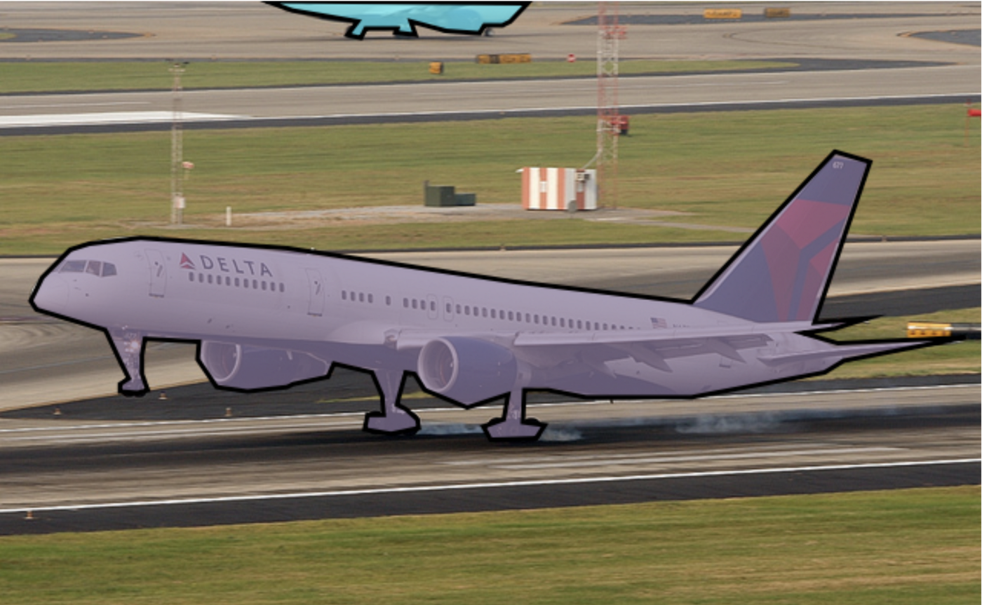
Let’s start with an intuitive explanation of the flow. Let T be an invertible transformation function and I an image, such that I’ = T(I) and T⁻¹(I’) = I. Let S be the segmentation function, in our case the neural network, which outputs a probability map for each class of the image. Assuming that the image is split in Background, Ground and Sky and its size is W × H, the output of the network would be 3 matrices of size W × H with per-pixel probabilities, for each of the previously mentioned classes. The class with the highest probability of a pixel is the chosen class for it. Thus, we segment the image into 3 classes.

Traditionally, as also mentioned before, people would spend lots of hours annotating a huge training set, setting the class for each pixel, which should be both consistent and correct. You can imagine how much time it takes to annotate an image. Multiply this with 40.000. That’s the number of images for the smallest dataset this paper handles, namely CocoStuff3.

As a reader, you might wonder how is someone able to take pictures with these 3 classes only. With a very high probability, any image will contain some other classes, be it humans, cars, or buildings. On top of the annotation work, labelers must also define a mask, that covers all the non-stuff classes. This must be a lot of work.

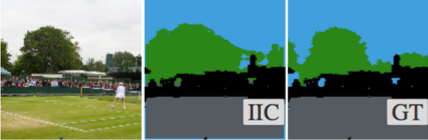
Real image — result of the network — segmentation by a human.

Going back to our T, S and I, the method proposed by the authors of the paper is to take the image I, build a geometrically transformed image I’ = T(I). Having this, predict the per-pixel probabilities for each, P = S(I) and P’ = S(I’), then expect that, by reverting all the geometrical transformations of the latter to get similar results: P ≈ T⁻¹(P’).

This leads us to the next section, namely mutual information.

Mutual Information and Paired Data

As briefly introduced before, you might already have a feeling that we handle paired data. Although this learning framework should learn on any generic paired dataset (which will touch on later), it presents the specific case of using pairs of images. The idea is to make the network learn what is common between semantically similar images and what differs between different images. This is called mutual information:

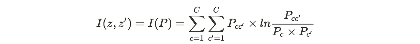
Confusing, right? Let’s break it down. For the simpler clustering use case, there is one prediction per image, for each of the classes C. If we take a pair of images and combine their predictions we get P ∈ C×C, a matrix with all the probability combinations. In fact, Pcc’ = P(z=c, z’=c’) and Pc is the sum of that specific column, ∑ Pcc’ . If we take two cat images, we would expect them to share the same mutual information, thus having a high P cat cat’, maximizing the mutual information I. But we said that we don’t manually annotate or pair images, which is true.

The image pairs are generated automatically, by taking the original image and a perturbed version of it, which does not break the content. We can use color filters, blur and revertible geometrical transformations. The idea is that, if we have a cat image and the same cat image rotated at 90°, we expect that their output is the same if rotating the latter back.

How does clustering work?

Taking the image pairs from previous chapters + the mutual information function, we end up with more or less a classification algorithm. If we manage to make the model learn which is what cars have in common and what cats have in common, using automatically generated pairs, we have a pretty solid base for generalizing how many classes we want.

There is also a twist. Some data might come into 2 buckets: simple and clean or filled with distractor classes. We can train our model on the first, but also introduce an auxiliary overclustering head, which would learn to classify, maybe with lower accuracy, the noisy data. This way, our simple classifier will benefit by looking, with another pair of eyes to a more cluttered image. It is like a student would study for a super hard problem, just to help to get better at a hard one.

How does segmentation work?

Generalizing even more, if we take the per-image clustering to per-patch clustering, we eventually converge to per-pixel clustering, which is indeed image segmentation. We assign each pixel a class and thus we separate the entities. To make this generic enough, and not just a random per-pixel prediction, they do this for neighboring patches, so that they also include spatial relationships. You can think of all this operation more or less like a convolution, which takes a patch and returns a value (in our case, one probability value per predicted class C.

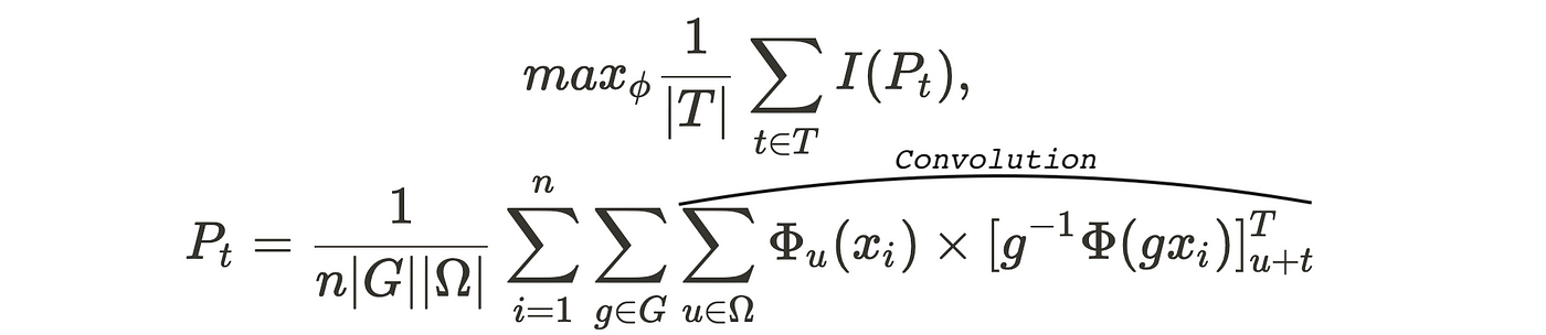
First of all, let’s break down this monolith. The convolution part is computing the mutual information, the first term of the product is the prediction on the original image and the second is the un-transformed prediction for the transformed original image. The summing terms in the front go over batches and image patches, while P_t is scaled with the size of the batch and the total number of patches. Now it should be a bit more clear.

Mutual information as a loss function

We have defined the data model, the function that tells us how good the model is performing, but how do we make it learn. We have to transform the mutual information score into a loss function. Since it already predicts a ‘loss’ value per pixel, it is directly a good measure of the performance.

Mutual information expands to I(z, z’) = H(z) − H(z|z’). Hence, maximizing this quantity trades-off minimizing the conditional cluster assignment entropy H(z|z’) and maximizing individual cluster assignments entropy H(z). The smallest value of H(z|z’) is 0, obtained when the cluster assignments are exactly predictable from each other. The largest value of H(z) is lnC, obtained when all clusters are equally likely to be picked. This occurs when the data is assigned evenly between the clusters, equalizing their mass. Therefore the loss is not minimized if all samples are assigned to a single cluster (i.e. output class is identical for all samples). Thus as maximizing mutual information naturally balances reinforcement of predictions with mass equalization, it avoids the tendency for degenerate solutions (predicting only one class).

The learning flow

As you might guess, the flow starts with loads of unlabeled images, intending to create a segmentation mechanism without much annotation work. After loading batches of data sequentially, some random transformations are chosen and saved for future undo-ing. Then, the learning flow follows more or less a conventional path, with sequences of data flowing forward and the mutual information loss adjusting the weights as it goes backward through the network. This is, on a very high level, the whole learning flow, showing once again how easy it can be to learn from automatically generated pairs of data, validating their mathematical assumption that mutual information, indeed, works.

One interesting thing to note is that, since they don’t have the true labels of their segments, they perform a matching between their patches and the ones in the test set, building thus the permutation that behaves best when checking the model’s performance.

Beating all the SOTAs

This piece of research is important from a particular point of view: it outperforms the previous state of the art in many areas and challenges. The novel architecture shows better scores in various datasets, STL, CIFAR, MNIST, COCO-Stuff, and Potsdam being among them. Moreover, it beats them with a significant margin.

72.3%

You would generally say that 72.3% is a pretty bad accuracy. Think twice. We, as humans, have a pretty good perception of depth, but often find it hard to distinguish between objects far away and sky for example, or between grass and bushes in the background. Given that a computer vision model, trained with 0 supervision achieves this performance is quite a leap forward towards better autonomous cars, more accurate robots, and safer AI systems in general.

Although they achieve this very nice score, there is a twist.

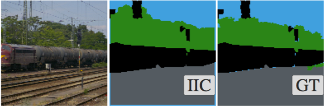
Look at this image, how many segmented classes do you see? 4, right? It should not be the case, because the model only knows to identify ground, sky, and background. Here comes the thing, they use a predefined mask that removes all the non-stuff content. They train the model on images for which the mask is no more than 25% of the image size. Although from a research perspective this is a very nice output and confirms the mathematical assumptions, the approach might not be directly usable in a real production setting. In an autonomous vehicle, there isn’t a mask on everything that’s not sky, background, and ground, so the model might find it hard to decide if a human is a human, or just an object far away. If we know that the real-life model receives an image with only those 3 classes, perfect, 72.3% accuracy guaranteed, but otherwise, there might be some issues related to predicting the masked pixels.

Replicating the paper

We rewrote parts of the code to make it more modular. This allowed us to make experiments easier and also train a model in the cloud from scratch. In just 12 hours we got an accuracy of 68%, pretty close to their 72.3% and we do believe that a few more hours would have already trained the model above 70%.

We thought of a little experiment, where we took the same test set, but excluded the mask totally, just to get a sense of how well the model will perform in the real world. Since the mask is at most 25% of the image, which is bonus points given to the classifiers, we expect a real-life accuracy ∈ [47.3%, 72.3%]. Since the metric cannot be computed in a deterministic way (we have to choose some subjective rules for predicting the mask), we decided not to pursue this path ahead, since the numbers can be randomly in the previous interval. The model is learned to ignore the mask pixels altogether, so we felt there is not much value to be derived from an accuracy retrieved from an arbitrary heuristic.

The paper presents a method that might be the stepping stone for further research on this topic, where state of the art results can be achieved without manual labeling. We see as future research the same technique applied to semantically segment sentences or even sequences of videos.

With a 72.3% accuracy on CocoStuff3, the Invariant Information Clustering for Unsupervised Image Classification and Segmentation paper demonstrates that state of the art results can be achieved with a simple model, but deep mathematical intuition.

This post builds upon the work of Xu Ji, João F. Henriques and Andrea Vevaldi in the IIC paper while you can find the modified code here.